Research Question

Can Engineered Market Signals Identify Future Relative Outperformers?

Research objective and study context.

Systematic portfolio management is fundamentally a ranking problem. Investors rarely need to predict the exact return of every asset; instead, they need to identify which assets are most likely to outperform their peers over a future investment horizon.

This research investigates whether engineered market signals can be used to identify future relative outperformance across a diversified ETF universe. Rather than forecasting absolute market direction, the objective is to rank assets according to their expected future risk-adjusted performance and determine whether persistent cross-sectional structure exists within financial markets.

Why This Question Matters

Financial markets exhibit persistent trends, changing volatility regimes, temporary dislocations, and evolving cross-asset relationships. If these behaviours leave measurable patterns in historical data, they may provide information about future relative performance.

Understanding whether such information exists is a fundamental problem in quantitative investing because portfolio construction ultimately depends on identifying relative winners and losers rather than accurately forecasting the direction of the overall market.

Key Takeaway

The objective is not to predict market direction. The objective is to determine whether market observations contain sufficient information to identify the assets most likely to outperform their peers on a risk-adjusted basis over the next five trading days.

Transition

Having defined the research question, the next step is to establish how the investigation will be conducted. The following section introduces the research workflow and explains how market observations are transformed into predictions, portfolio decisions, and validated research findings.

Methodology

02 Research Design

How the investigation will be conducted.

A quantitative research result is only meaningful if the process that produced it is transparent, reproducible, and free from look-ahead bias. This investigation therefore follows a structured workflow that separates data preparation, prediction, portfolio construction, historical evaluation, and validation into distinct stages.

The objective is not simply to train a model and report a performance metric. Instead, the goal is to evaluate an entire research process, beginning with raw market observations and ending with validated portfolio behaviour.

Workflow Architecture

Market observations to validated findings

  1. DataSection 03
    • 01Market Prices
    • 02Feature Construction
  2. PredictionSection 04
    • 03Prediction Model
    • 04Asset Rankings
  3. PortfolioSection 05
    • 05Portfolio Construction
  4. EvaluationSections 06–07
    • 06Backtesting
    • 07Validation
  5. FindingsSections 08–09
    • 08Research Findings & Limitations
Figure 02. Phase-based workflow architecture showing how market observations move through data preparation, prediction, portfolio construction, evaluation, and learning before research conclusions are drawn.
Workflow Description

From Observations To Research Conclusions

The workflow begins with daily market observations collected across a diversified ETF universe. These observations are transformed into engineered features representing different hypotheses about market behaviour. A prediction model converts the feature set into cross-sectional forecasts, producing a ranking of assets according to expected future performance.

Forecasts are translated into portfolio allocations through a systematic portfolio construction process. The resulting portfolio is evaluated through historical simulation under explicit transaction-cost assumptions before being subjected to walk-forward validation. Only after the full process has been completed are conclusions drawn regarding predictive behaviour, robustness, and practical implementation.

Why This Design?

Chronology, Alignment, And Execution Assumptions

The design deliberately aligns prediction horizon, target construction, and portfolio implementation. Forecasts target a five-day investment horizon, positions are held for five trading days, and portfolio turnover is evaluated under explicit transaction-cost assumptions.

This alignment ensures that predictive signals are assessed under realistic execution conditions rather than in isolation.

The workflow also enforces strict chronology. Information available at the time of prediction is separated from future observations used for evaluation, ensuring that every stage of the research process reflects the information that would have been available historically.

Key Takeaway

The showcase evaluates a complete quantitative research process rather than a single predictive model. Every result presented in later sections is produced through a structured workflow that preserves chronology, incorporates execution assumptions, and separates model development from out-of-sample validation.

Transition

Having established the research workflow, the next step is to examine the information available to the prediction system. The following section introduces the engineered feature library and explains how market observations are transformed into quantitative signals.

Data & Feature Construction

03 From Market Observations to Quantitative Signals

Feature engineering and target construction.

Market prices do not directly reveal future opportunities. They provide only a historical record of how assets have behaved through time. The central challenge of quantitative research is therefore not collecting data, but transforming observations into information that may contain predictive value.

This investigation approaches that problem through systematic feature engineering. Rather than presenting raw prices to the prediction model, historical market behaviour is translated into a structured feature library designed to represent different hypotheses about how assets behave across market environments.

The objective is not to identify a single indicator capable of predicting future returns. Instead, the feature set intentionally combines multiple perspectives on market behaviour, allowing the model to evaluate trend persistence, volatility conditions, mean-reversion pressure, and broader market structure simultaneously.

The result is a feature space that attempts to capture how assets differ from one another at any point in time, creating the foundation for cross-sectional ranking and portfolio construction.

03.1

Cross-Asset Environment

Before constructing predictive signals, it is important to understand the environment in which the model operates.

The research universe contains twenty ETFs spanning equities, fixed income, commodities, credit, real estate, and defensive sectors. The purpose of this diversification is not merely to increase the number of assets. Cross-sectional prediction requires meaningful differences between assets. If all instruments moved identically through time, there would be no ranking problem to solve.

The correlation structure therefore provides a first view of the opportunity set available to the model.

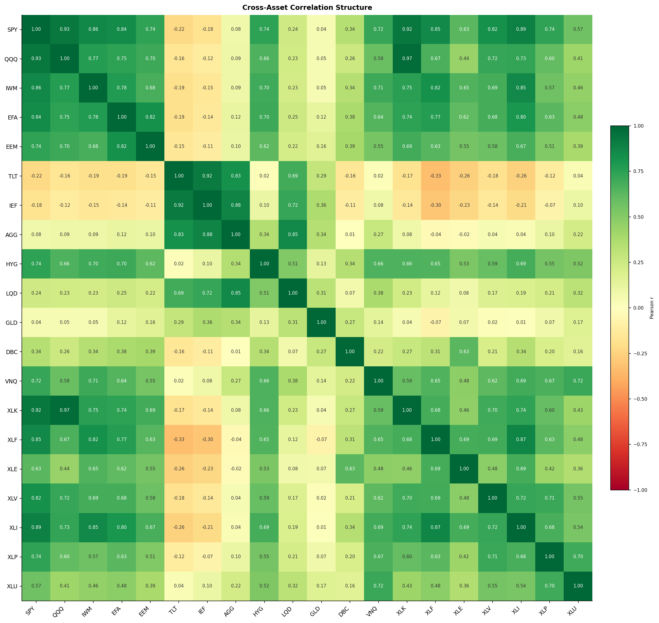
Cross-asset return correlation heatmap for the twenty ETF research universe.
Figure 03.1 - Cross-Asset Correlation Structure. Universe correlation heatmap.

The figure reveals several distinct clusters. Equity ETFs exhibit strong positive correlation, reflecting shared exposure to economic growth and investor risk appetite. Fixed-income instruments form a separate cluster, while commodities and precious metals display weaker relationships with traditional risk assets.

These differences are important because they create the variation required for cross-sectional prediction. The objective of the model is not to forecast whether markets will rise or fall, but to identify which assets are likely to outperform their peers over a defined investment horizon.

03.2

Feature Engineering Framework

Having established the cross-asset environment, the next step is to determine what information should be extracted from market observations.

A single feature rarely captures the full complexity of market behaviour. Signals that perform well during trending markets often deteriorate during volatile or mean-reverting environments. To reduce dependence on any single market hypothesis, the feature library combines signals from four complementary feature families.

Feature Family

Research Objective

Feature FamilyResearch Objective
TrendCapture persistence and continuation of relative leadership
VolatilityCharacterise changing risk environments
Mean ReversionMeasure distance from equilibrium conditions
Market StructureCapture systematic market exposure

Trend-oriented features form the largest component of the library. This reflects the central research question of the investigation: whether persistent cross-sectional leadership can be identified and exploited across a diversified ETF universe.

The final feature library contains fifteen engineered signals spanning these four research themes.

03.3

Feature Inventory

Each feature represents an explicit hypothesis regarding future cross-sectional performance.

Rather than relying on opaque transformations, every signal has a clear economic interpretation and a corresponding research rationale.

Feature Inventory

Fifteen engineered signals

FeatureFamilyDescriptionResearch Hypothesis
5D MomentumTrendRecent five-day returnShort-term continuation may persist
20D MomentumTrendOne-month returnIntermediate leadership may continue
60D MomentumTrendThree-month returnSustained trends may remain intact
252D MomentumTrendOne-year returnLong-term winners may continue outperforming
20D Trend StrengthTrendConsistency of directional movementStrong trends outperform weak trends
20D Trend PersistenceTrendFraction of positive daysConsistent advances outperform noisy advances
63D Breakout StrengthTrendDistance from recent highsAssets near highs may continue higher
63D Risk-Adjusted MomentumTrendReturn adjusted for volatilityEfficient trends outperform volatile trends
126D Risk-Adjusted MomentumTrendMedium-term risk-adjusted trendPersistent efficient leadership
252D Risk-Adjusted MomentumTrendLong-term risk-adjusted trendStructural outperformance persists
21D Realised VolatilityVolatilityRecent realised riskRisk conditions contain predictive information
Volatility Compression (21D/63D)VolatilityShort versus long volatility ratioCompression may precede regime expansion
20D Z-ScoreMean ReversionDistance from recent meanExtreme moves may revert
252D Drawdown DistanceMean ReversionDistance from annual peakDeep drawdowns may recover
60D Market BetaMarket StructureSensitivity to market movementsSystematic exposure influences relative performance

Together, these features transform raw price observations into a structured representation of market behaviour that can be evaluated by the prediction model.

03.4

Feature Relationships

Once the feature library has been constructed, it is important to understand how the signals relate to one another.

Complete independence is neither realistic nor desirable. Features designed to measure similar market phenomena are expected to share information. The objective is not to eliminate correlation entirely, but to ensure that multiple market hypotheses are represented within the feature space.

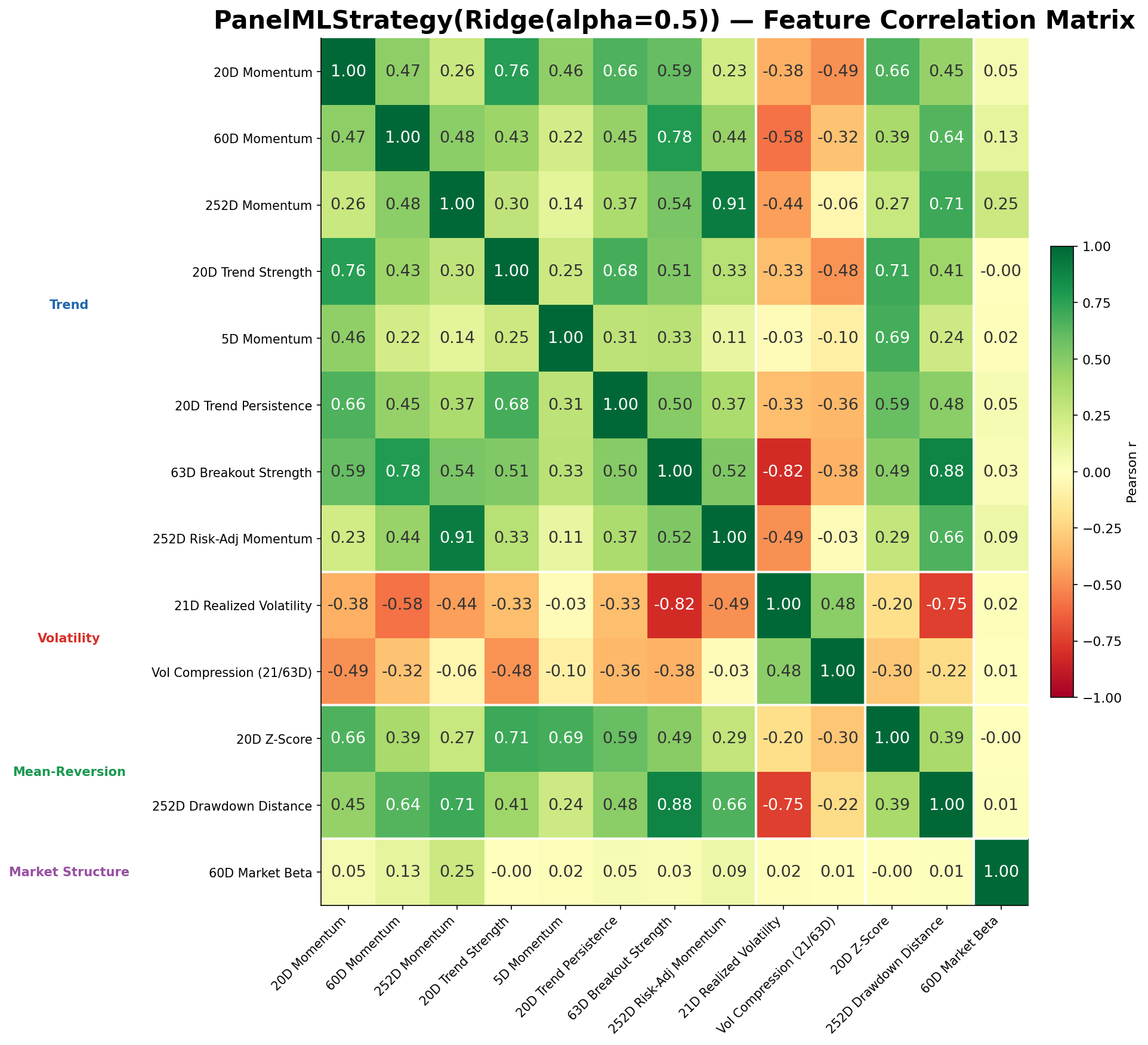
Feature correlation heatmap showing relationships among the fifteen engineered signals.
Figure 03.2 - Feature Correlation Matrix. Feature correlation heatmap.

Several momentum-based features exhibit strong positive relationships, particularly among long-horizon trend signals and their risk-adjusted counterparts. This behaviour is expected because these features attempt to describe related aspects of market persistence.

At the same time, volatility and market-structure features remain comparatively distinct. Market beta, for example, displays limited correlation with most other signals, suggesting that it contributes information not captured by traditional price-based trend indicators.

The resulting feature space therefore contains both intentional overlap and meaningful diversification, providing the model with multiple perspectives on market behaviour.

03.5

Feature Behaviour Through Time

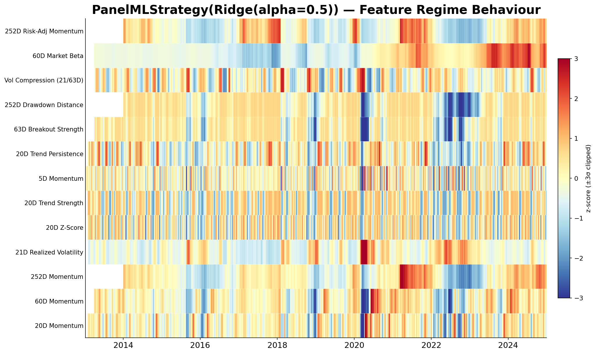
Feature definitions remain constant throughout the research period, but feature values do not.

Markets evolve continuously. Relationships that appear stable during one environment may weaken, strengthen, or reverse as conditions change. Understanding this evolution is therefore as important as understanding the features themselves.

Feature regime evolution heatmap showing engineered signal behaviour through time.
Figure 03.3 - Feature Regime Evolution. Feature regime evolution heatmap.

The figure tracks the behaviour of all fifteen features throughout the twelve-year research period. Several major market events are clearly visible, including the 2020 pandemic shock and the 2022 tightening cycle, both of which produced simultaneous changes across multiple feature families.

Trend features, volatility signals, and market-structure measures respond differently to these transitions, illustrating the non-stationary nature of financial markets.

This observation motivates a central design principle of the research process: predictive signals must be evaluated across multiple market environments rather than within a single historical period. The same feature can exhibit very different behaviour depending on the regime in which it is observed.

03.6

Target Construction

Features define the information available to the model. The prediction target defines what the model is attempting to learn.

Rather than forecasting absolute future returns, the investigation focuses on a cross-sectional ranking problem. The objective is to identify which assets are likely to outperform their peers over the next investment horizon.

The prediction target is constructed in three stages.

  1. Step 1

    Future Return

    For every asset, the forward five-day return is calculated.

  2. Step 2

    Risk Adjustment

    The forward return is adjusted for realised volatility over the same horizon. This rewards assets that generate returns efficiently rather than simply taking greater risk.

  3. Step 3

    Cross-Sectional Ranking

    Assets are ranked against one another according to their future risk-adjusted performance. The highest-ranked assets become positive training examples, while the lowest-ranked assets become negative training examples.

The resulting label is therefore a five-day risk-adjusted cross-sectional ranking target rather than a conventional return forecast.

This design aligns the prediction objective with the eventual portfolio construction process, where assets are selected relative to one another rather than evaluated in isolation.

03.7

Alignment and Leakage Prevention

A quantitative research process is only credible if the information available at the time of prediction remains strictly separated from future observations.

All features are constructed exclusively from historical information available at time t. Labels are constructed using information that occurs after time t. The two are aligned only after both processes have been completed.

The longest feature requires a 252-trading-day lookback window, creating an initial warm-up period before valid observations become available. An additional five trading days are required to construct forward labels.

These observations are removed prior to model training.

Key Takeaway

As a result, every sample presented to the model reflects information that would have been genuinely available at that point in history, ensuring that subsequent analysis remains free from look-ahead bias.

Transition to Section 04

Having transformed market observations into a structured feature space and constructed a leakage-safe prediction target, the next stage is to determine whether a prediction model can learn useful relationships between these signals and future cross-sectional performance.

Modelling

04 From Signals to Forecasts

How engineered signals are transformed into forecasts.

04.1

From Features to Forecasts

Section 03 established the information available to the prediction system. Daily market observations were transformed into fifteen engineered features representing trend, volatility, mean reversion, and market structure hypotheses. A five-day risk-adjusted ranking target was then constructed to represent future cross-sectional performance.

The next question is whether a statistical model can learn a relationship between these inputs and future outcomes.

Financial forecasting presents a fundamentally different challenge from many machine-learning applications. Market returns are noisy, relationships evolve through time, and predictive signals are often weak relative to random fluctuations. The objective is therefore not simply to fit historical data, but to identify relationships that remain informative under changing market conditions.

This section examines how the prediction system is constructed and evaluates whether the resulting forecasts contain meaningful cross-sectional information before any portfolio decisions are made.

04.2

Why Ridge Regression?

A prediction model must balance two competing objectives.

On one hand, the model must be flexible enough to detect subtle relationships within noisy financial data. On the other, excessive flexibility increases the risk of fitting historical noise rather than genuine market structure.

For this investigation, Ridge Regression was selected as the primary forecasting model. Ridge extends ordinary linear regression through L2 regularisation, penalising excessively large coefficients and encouraging more stable parameter estimates. The approach is intentionally simple, transparent, and interpretable, allowing the research to focus on whether the feature library itself contains predictive information.

Rather than treating the model as a black box, the objective is to use a disciplined baseline that provides visibility into the relationship between engineered signals and future outcomes.

Prediction Model Configuration

Ridge forecasting setup

ParameterValue
ModelRidge Regression
RegularisationL2
Alpha1.0
Features15
Assets20
Forecast Horizon5 Trading Days
Retraining Frequency30 Trading Days
04.3

A Panel Learning Framework

Instead of training a separate model for each ETF, all observations are pooled into a single panel dataset.

Each training sample represents a specific asset on a specific date:

Input Unit(Date, Asset)
Feature Vector15 Engineered Features
Learning TargetFuture Risk-Adjusted Rank

This design allows the model to learn relationships that generalise across the entire universe rather than memorising behaviour within individual assets.

The resulting prediction system continuously evaluates relative opportunities across equities, bonds, commodities, credit, real estate, and defensive sectors using a shared set of learned relationships.

Importantly, the model does not directly produce buy or sell decisions. The output is a forecast score for every asset at each rebalance date. These scores form the foundation of the ranking system examined below.

04.4

Measuring Predictive Information

Before forecasts can be converted into portfolio allocations, it is necessary to determine whether the prediction scores contain useful information.

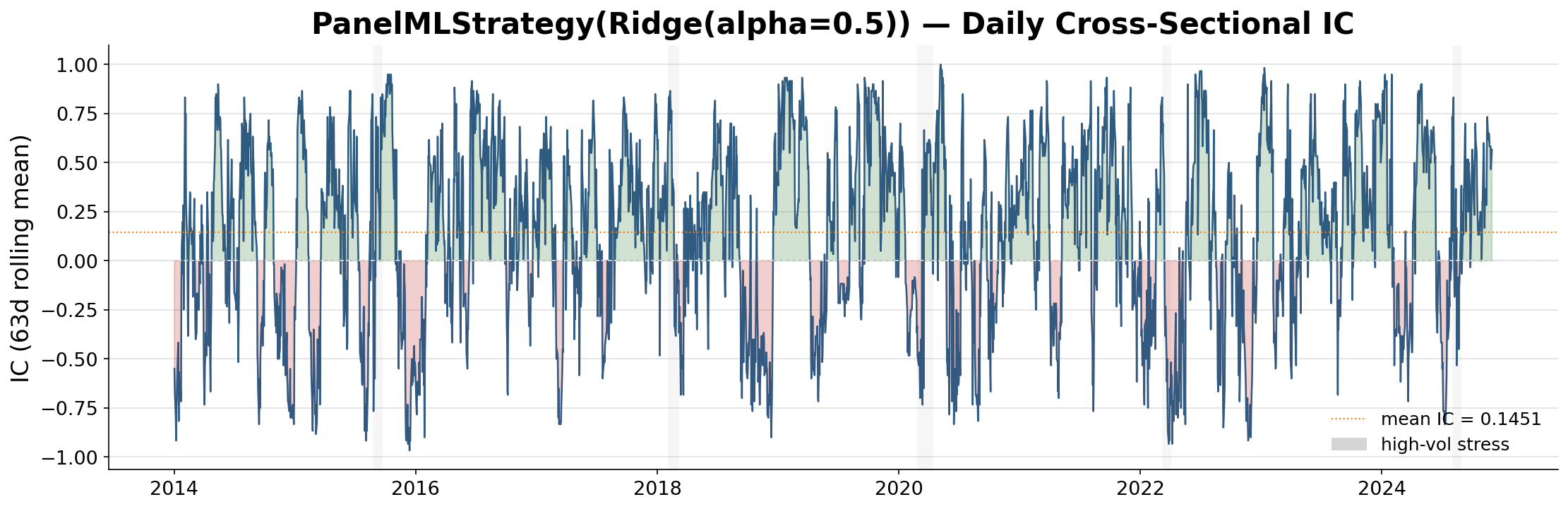
The first diagnostic examines the relationship between predicted rankings and realised future rankings. This relationship is measured using the Cross-Sectional Information Coefficient (IC), a standard quantitative research metric that evaluates whether assets assigned higher scores subsequently outperform assets assigned lower scores.

A positive IC indicates that the ranking system is directionally correct. An IC near zero suggests that the forecasts contain little useful information.

Cross-sectional information coefficient over time for the prediction system.
Figure 04.1 — cross_sectional_ic.

The Information Coefficient evaluates ranking quality rather than investment performance. Positive values indicate that assets receiving stronger predictions generally achieved stronger realised outcomes. Persistent positive observations suggest that the feature library contains information relevant to future cross-sectional performance.

The objective is not to predict exact returns, but to correctly identify which assets are likely to outperform their peers over the forecast horizon.

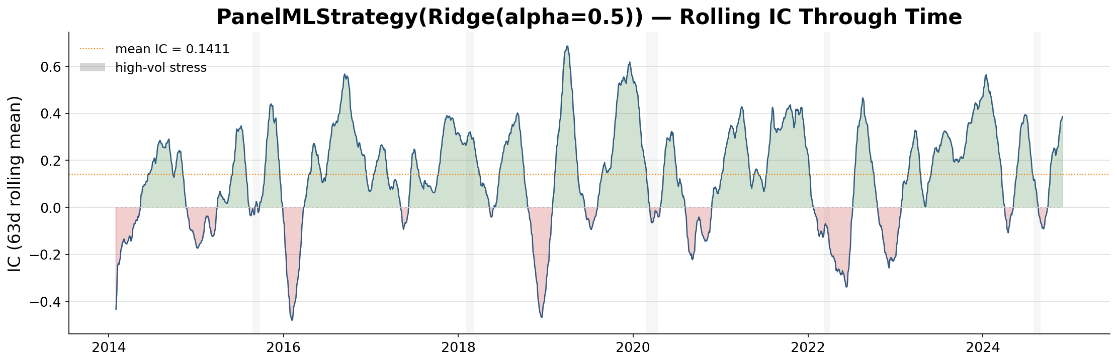
Forecast quality is rarely constant through time. Market relationships strengthen, weaken, and occasionally reverse as macroeconomic conditions evolve.

To understand how predictive information behaves across different environments, the Information Coefficient can be examined through time.

Rolling information coefficient regime diagnostic for forecast quality through time.
Figure 04.2 — ml_ic_regime.

The rolling IC highlights periods where predictive relationships strengthened and periods where signal quality deteriorated. Fluctuations are expected in financial forecasting, but persistent positive regions indicate that predictive information survives beyond isolated market episodes.

Rather than evaluating a single average value, the figure reveals how the forecasting system responds to changing market environments and provides an early indication of regime dependence.

04.5

From Predictions to Rankings

Demonstrating predictive information is only the first step.

The practical objective of the model is not to predict exact returns. The objective is to rank assets according to expected future attractiveness.

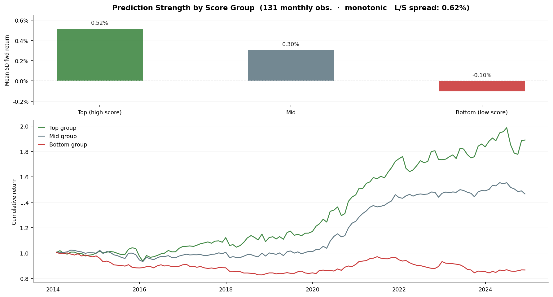
A useful ranking system should exhibit monotonic behaviour: assets receiving stronger predictions should, on average, achieve stronger future outcomes than assets receiving weaker predictions.

The following analysis evaluates whether prediction strength corresponds to realised performance.

Prediction strength diagnostic comparing realised outcomes across prediction groups.
Figure 04.3 — prediction_strength.

Assets assigned to higher prediction groups consistently achieve stronger realised forward returns than assets assigned to lower prediction groups. This monotonic ordering suggests that forecast magnitude carries meaningful information rather than acting as random noise.

The importance of this result is that the model is not merely separating assets arbitrarily. Stronger forecasts correspond to stronger realised outcomes, providing evidence that prediction scores contain economically meaningful information.

Importantly, this figure evaluates the quality of the ranking system itself rather than the profitability of a trading strategy.

04.6

Ranking Structure and Stability

A ranking system may appear predictive while still being difficult to implement in practice.

For example, forecasts may fluctuate excessively, rankings may change randomly between periods, or the separation between assets may be too small to support meaningful portfolio decisions.

The final diagnostics therefore examine the structure of the ranking system itself.

The objective is to determine whether the model consistently differentiates between opportunities, whether those differences are economically meaningful, and whether rankings remain stable through time.

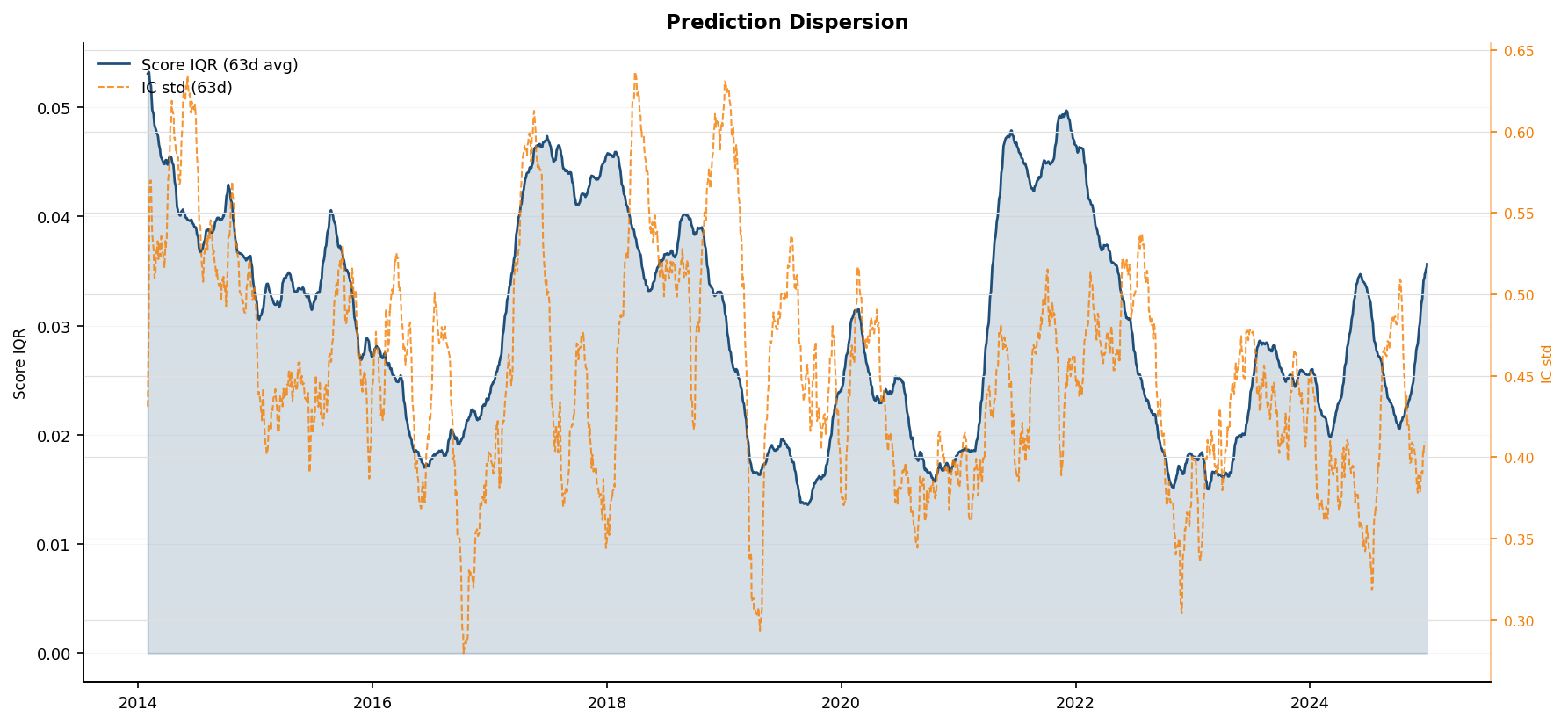
The interquartile range of prediction scores measures the degree of separation between assets. Larger values indicate stronger differentiation, while values approaching zero suggest that the model sees little distinction between available opportunities.

Interquartile range of prediction scores measuring cross-sectional ranking separation.
Figure 04.4ranking_geometry_iqr.

Persistent positive dispersion indicates that the forecasting system continues to identify relative differences between assets throughout the sample.

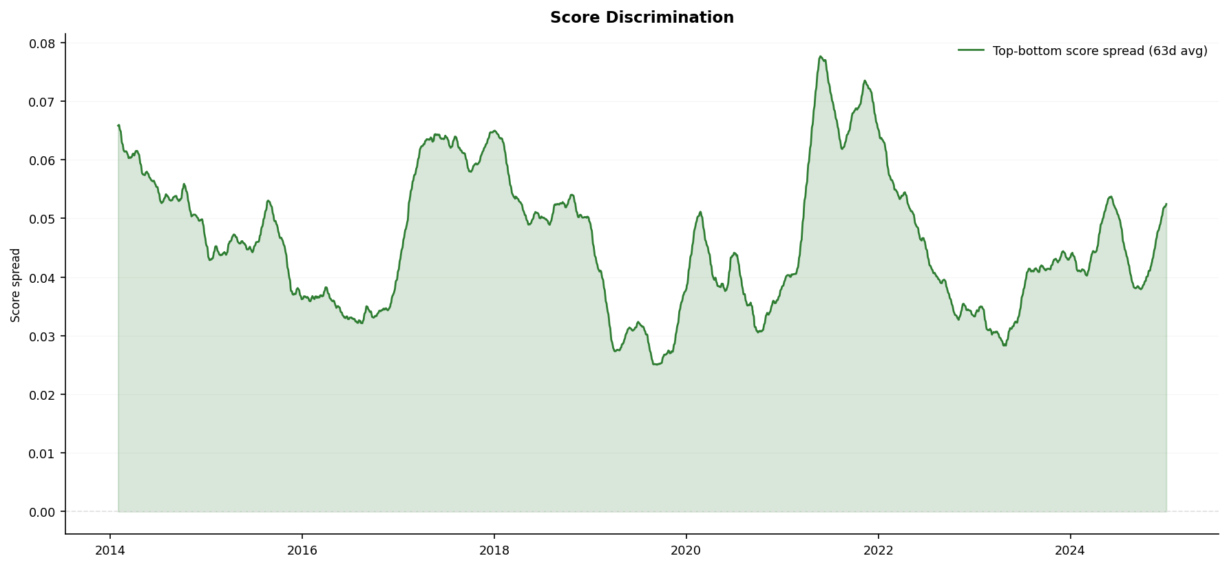
The top-versus-bottom score spread measures the distance between the model's strongest and weakest convictions.

Top-versus-bottom prediction score spread measuring model conviction through time.
Figure 04.5ranking_geometry_spread.

Large spreads indicate periods where the model expresses clear preferences. Smaller spreads indicate lower conviction and a reduced distinction between opportunities. This diagnostic provides a direct view of forecast confidence at the cross-sectional level.

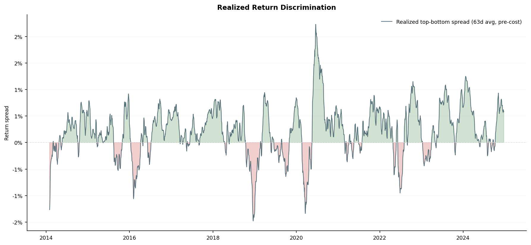
Prediction quality ultimately depends on whether score separation translates into outcome separation.

Realised performance spread between highest-ranked and lowest-ranked assets through time.
Figure 04.6ranking_geometry_realized.

This figure compares realised performance between the highest-ranked and lowest-ranked assets through time. Positive realised spreads indicate that stronger forecasts were associated with stronger outcomes. The diagnostic therefore provides a direct connection between prediction rankings and realised economic behaviour.

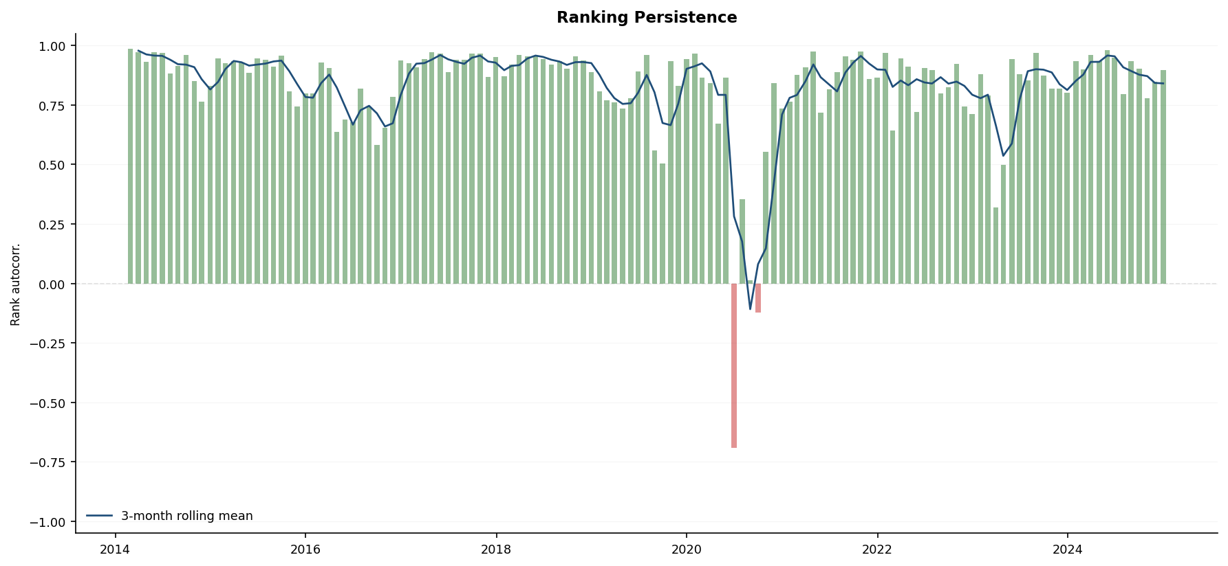
A useful ranking system should evolve gradually rather than changing randomly at every rebalance date.

Rank persistence diagnostic measuring stability of asset rankings between rebalance dates.
Figure 04.7ranking_geometry_persistence.

Rank persistence measures the stability of the model's convictions through time. Higher persistence indicates that the system maintains a consistent view of relative opportunities, while lower persistence suggests frequent reordering of the asset universe. Stable rankings are generally more interpretable and more practical to implement than rankings that fluctuate unpredictably between periods.

Key Takeaway

Section 03 demonstrated how market observations can be transformed into a structured feature library and a leakage-free prediction target. Section 04 demonstrates that these signals can be converted into forecasts that contain measurable cross-sectional information and produce economically meaningful asset rankings.

Transition to Section 05

The prediction system therefore provides a disciplined mechanism for identifying relative opportunities across the investment universe. The next stage of the research process is determining how these rankings are translated into portfolio allocations and investable positions.

Portfolio Construction

05 From Forecasts to Investment Decisions

05.1

From Prediction to Portfolio

The objective of the prediction system was not to generate forecasts for their own sake, but to determine whether the engineered feature library contained information that could be used to rank assets according to future performance. The diagnostics presented in the previous section provided evidence that the model's rankings were economically meaningful: higher-ranked assets generally outperformed lower-ranked assets, cross-sectional information coefficients were persistently positive, and prediction strength exhibited broadly monotonic behaviour.

These findings do not prove that the model is profitable. They merely establish that the ranking system contains information beyond random ordering. Having demonstrated that the predictions are sufficiently informative to warrant further investigation, the next question becomes how those forecasts should be translated into investment decisions.

The prediction system produces a continuously updated ranking of twenty assets according to expected five-day risk-adjusted performance. Rankings alone, however, are not investable. A portfolio construction framework is required to convert these forecasts into positions, allocate capital, and define how frequently the portfolio should adapt to new information. The choices made at this stage determine not only what the portfolio holds, but also the diversification characteristics, implementation practicality, and ultimately the behaviour of the strategy itself.

05.2

Portfolio Construction Framework

The prediction system produces rankings rather than investment decisions. Portfolio construction converts those rankings into positions.

At each rebalance date, all twenty assets are ranked according to their predicted five-day risk-adjusted performance. The five highest-ranked assets are selected for inclusion in the portfolio and allocated equal capital weights.

This design balances concentration and diversification. Holding a single asset would maximise conviction but make outcomes highly sensitive to prediction errors. Conversely, holding a large proportion of the universe would dilute the ranking signal and reduce the distinction between preferred and non-preferred assets. Selecting five assets concentrates capital in the model's highest-conviction opportunities while maintaining diversification across multiple holdings.

Equal weighting was chosen as a simple and robust allocation scheme. Although the prediction system demonstrated meaningful ranking ability, the magnitude of prediction scores was not perfectly calibrated. Allowing rankings to determine asset selection while distributing capital equally reduces sensitivity to estimation error and keeps the portfolio construction process transparent.

The forecast horizon and rebalance schedule are intentionally aligned. Predictions target five trading days ahead, and the portfolio is rebalanced every five trading days, ensuring that forecasts are evaluated over the horizon for which they were generated.

Portfolio Configuration

Portfolio Configuration

Asset Universe20 ETFs
Portfolio SizeTop 5 Assets
Weighting SchemeEqual Weight
Forecast Horizon5 Trading Days
Rebalance Frequency5 Trading Days
Model Retraining Frequency30 Trading Days
Transaction Cost Assumption5 bps
05.3

Portfolio Composition Through Time

The construction rules define how the portfolio should behave in theory. The next question is whether the resulting portfolio actually adapts to changing market conditions in practice.

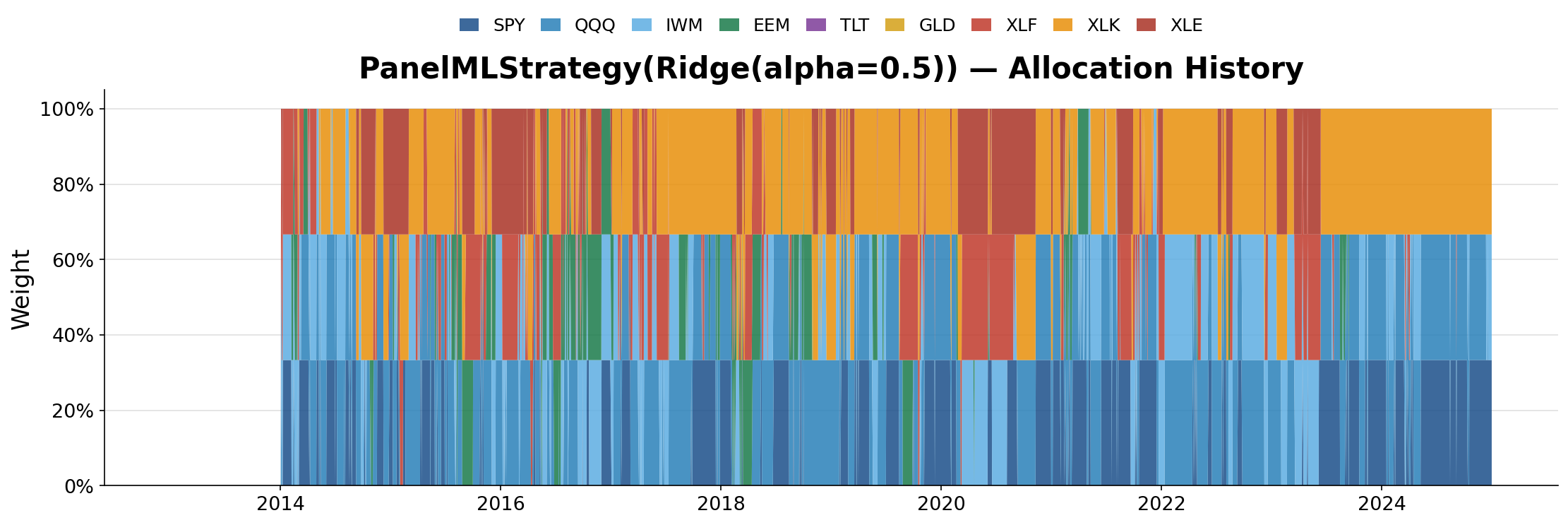
Portfolio allocation history showing selected ETF holdings through time.
Figure 05.1 - Portfolio composition through time. Each colour represents one of the selected holdings. Changes in composition reflect the model's response to evolving market conditions and illustrate how rankings are translated into investment decisions.

Figure allocation_history shows the realised portfolio composition throughout the research period. Each coloured band represents an asset held within the portfolio, allowing the evolution of allocations to be observed through time.

The portfolio is dynamic rather than static. As the prediction system updates its rankings, assets enter and leave the selected basket in response to changing market conditions. Periods dominated by growth-oriented assets differ substantially from periods in which defensive assets become more prominent, illustrating how the ranking system adapts to changing market environments.

More importantly, this figure represents the first observable output of the complete research pipeline. The feature library generates signals, the prediction system produces rankings, and the portfolio construction framework converts those rankings into actual investment decisions. What appears here is no longer a statistical forecast but an investable portfolio expressing the model's view of the market.

05.4

Portfolio Turnover

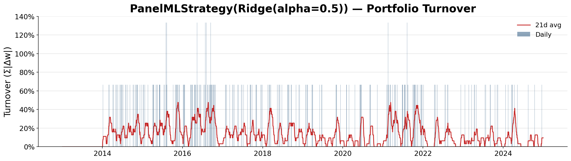
Adapting to new information requires trading. As rankings change, existing positions may be replaced by newly preferred assets, generating portfolio turnover.

Portfolio turnover through time showing changes in holdings at rebalance dates.
Figure 05.2 - Portfolio turnover through time. Higher values indicate more frequent changes in portfolio holdings and greater implementation activity, while lower values reflect more stable rankings and reduced trading requirements.

Figure portfolio_turnover shows the magnitude of portfolio changes through time. Periods of elevated turnover indicate environments in which rankings changed rapidly, requiring more frequent portfolio adjustments. Lower turnover suggests greater stability in the prediction system and lower implementation activity.

Turnover provides an important perspective on the practical behaviour of the strategy. A portfolio that continually changes its holdings may respond more quickly to new information, but it also requires more trading activity to maintain exposure to the model's preferred opportunities. Conversely, stable rankings lead to lower turnover and a more persistent portfolio structure.

Viewed together, the allocation and turnover figures reveal how the prediction system behaves once deployed as an investment process: which assets are selected, how frequently those selections change, and how actively the portfolio adapts to new information.

Key Takeaway

The prediction system identifies opportunities, but portfolio construction determines how those opportunities are expressed in practice. By selecting the five highest-ranked assets, allocating capital equally across positions, and rebalancing every five trading days, the research converts statistical forecasts into a transparent and implementable investment process.

The resulting portfolio remains focused on the model's highest-conviction opportunities while maintaining diversification across multiple holdings. The allocation history reveals how the strategy adapts to changing market conditions, while turnover quantifies the level of trading activity required to maintain those exposures.

Transition to Section 06

Having established how forecasts become positions, the next step is to evaluate how this portfolio would have behaved when traded through historical market conditions.

Performance Evaluation

06 Historical Strategy Performance

06.1

Evaluating the Complete Research Process

The preceding sections established the individual components of the research framework. A diversified universe was selected, a feature library was engineered from historical price behaviour, a machine learning model was trained to generate cross-sectional rankings, and those rankings were translated into a systematic portfolio construction process.

Each stage was designed to answer a specific research question. Together, however, they form a single investment strategy. The ultimate test of the research process is therefore not whether the model can generate predictions, but whether those predictions can be transformed into attractive investment outcomes.

This section evaluates the historical performance of the complete system. The objective is not to determine whether the strategy is robust or production-ready. Rather, it is to establish whether the combination of feature engineering, prediction modelling, and portfolio construction generated economically meaningful results over the research period.

06.2

Performance Summary

The strategy was evaluated over the period from January 2013 to December 2024 using the portfolio construction framework described in the previous section.

Performance Metrics

Performance Metrics

Annualised Return11.12%
Annualised Volatility17.40%
Sharpe Ratio0.69
Max Drawdown-32.91%
Calmar Ratio0.34

Taken in isolation, these metrics suggest that the strategy generated positive long-term returns while maintaining a moderate level of risk-adjusted performance. However, summary statistics provide only a partial picture. Understanding how returns were earned, how risk evolved through time, and how the strategy behaved during periods of market stress requires a more detailed examination of the return path itself.

06.3

Capital Growth and Drawdowns

The ultimate objective of any investment strategy is not to maximise prediction accuracy but to generate attractive investment outcomes. The equity curve therefore provides the most direct assessment of whether the research process translated into economic value.

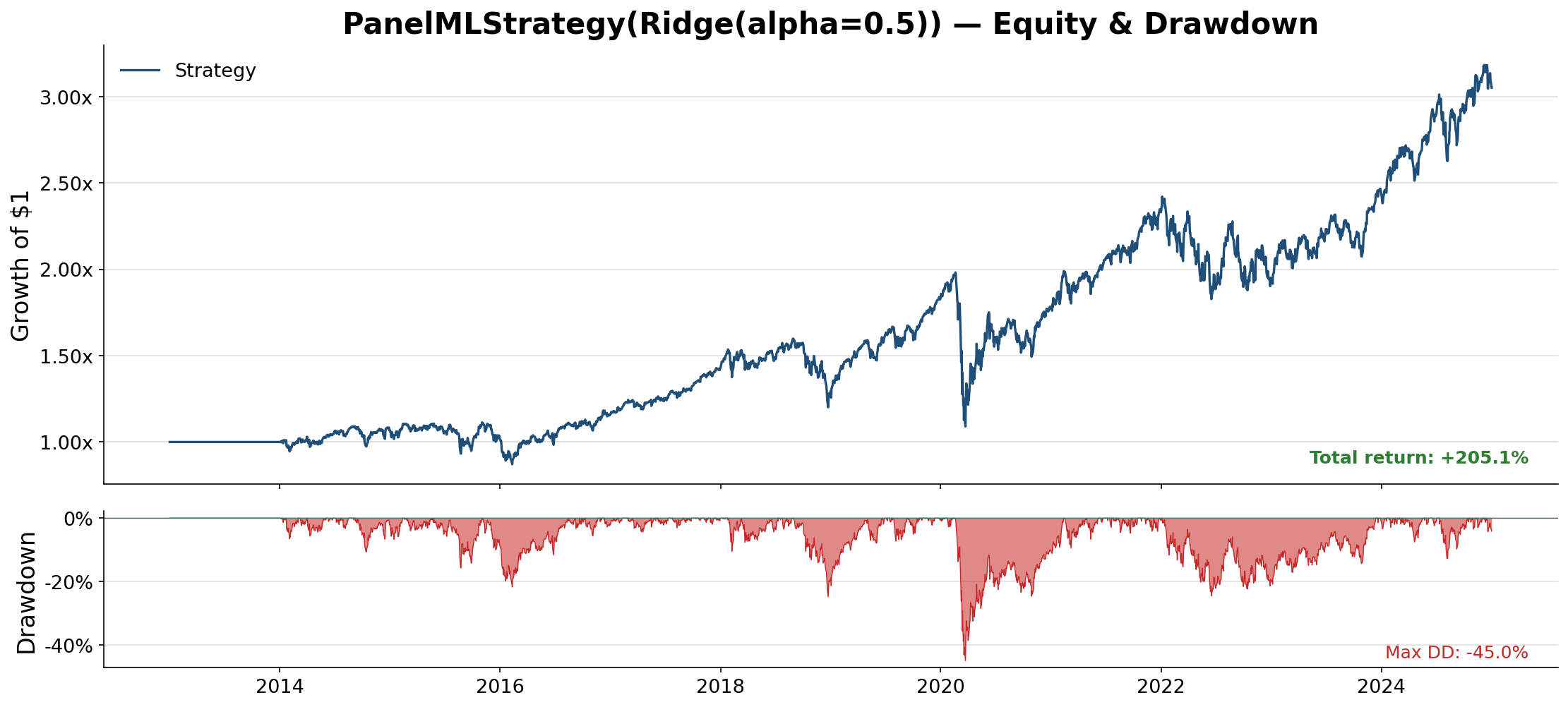
Equity curve and drawdown chart showing capital growth and peak-to-trough losses through time.
Figure 06.1 - Growth of one unit of capital alongside realised drawdowns from previous peaks. The strategy generated positive long-term growth but experienced several periods of material underperformance, illustrating the trade-off between return generation and risk exposure.

Figure equity_and_drawdown shows the growth of one unit of capital invested in the strategy throughout the research period, together with the associated drawdowns from previous equity peaks.

The portfolio generated positive long-term growth over the sample period, indicating that the prediction and portfolio construction framework was able to extract economically useful information from the underlying feature set. This result is particularly notable because the strategy relies exclusively on price-derived features and operates within a highly competitive market environment.

The path to that outcome, however, was not smooth. Several periods of material drawdown occurred throughout the backtest, reflecting changing market conditions and the inherent uncertainty associated with forecasting asset returns. The most severe drawdown reached approximately 33%, demonstrating that even profitable systematic strategies can experience prolonged periods of underperformance.

This observation highlights an important principle of quantitative investing. A strategy should not be judged solely by its cumulative return. The consistency of returns, the magnitude of losses, and the speed of recovery are equally important considerations when evaluating whether a research process produces economically meaningful results.

06.4

Performance Stability Through Time

While cumulative performance provides an overall assessment of success, it does not reveal whether that performance was generated consistently throughout the research period.

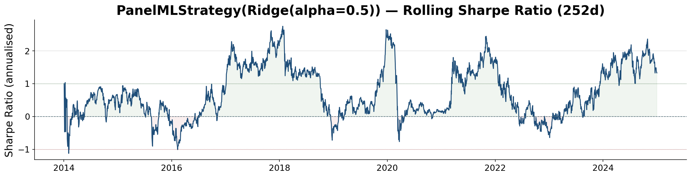
Rolling Sharpe ratio chart showing realised risk-adjusted performance through time.
Figure 06.2 - Rolling risk-adjusted performance through time. Periods of strong and weak performance reveal the extent to which strategy effectiveness varies across market regimes and provide insight into the stability of the underlying signal.

Figure rolling_sharpe shows the evolution of realised risk-adjusted performance through time. Positive values indicate periods in which returns were sufficiently large relative to realised volatility, while negative values identify periods of sustained underperformance.

The figure reveals that performance was regime dependent rather than uniformly distributed. Some market environments were considerably more favourable to the strategy than others, resulting in meaningful variation in realised risk-adjusted returns. This behaviour is consistent with the findings from earlier sections, where the effectiveness of features and prediction signals was shown to vary across different market conditions.

Importantly, periods of weaker performance do not necessarily invalidate the research hypothesis. Financial markets are inherently non-stationary, and systematic strategies frequently experience cycles of strength and weakness as market structure evolves. What matters is whether the strategy can generate positive outcomes across a sufficiently broad range of environments rather than succeeding in a single favourable regime.

The variability observed in the rolling Sharpe profile therefore motivates a deeper examination of robustness. A strong historical backtest is encouraging, but it does not by itself demonstrate that the underlying signal generalises beyond the specific periods in which it was observed.

Key Takeaway

The complete research process produced a portfolio that generated positive long-term returns and a positive risk-adjusted performance profile over the sample period. The results suggest that the feature engineering framework, prediction system, and portfolio construction process were collectively able to extract economically meaningful information from historical price data.

At the same time, the strategy experienced substantial drawdowns and meaningful variation in performance across different market environments. These observations highlight both the potential and the limitations of the research approach. Historical performance alone is insufficient to establish robustness.

A strong backtest demonstrates that the strategy worked under the conditions observed during the sample period. The next question is whether those results persist when the research process is repeatedly evaluated across independent out-of-sample windows. The following section therefore examines the robustness and consistency of the strategy using walk-forward validation.

Transition to Section 07

The historical results presented in this section provide evidence that the research framework generated economically meaningful performance over the full sample period. However, historical performance alone cannot determine whether the observed results reflect genuine predictive relationships or patterns that are specific to the data used during model development.

A strategy may appear successful in hindsight while failing to generalise when evaluated on genuinely unseen observations. Establishing whether the signal survives exposure to new market environments therefore requires a more rigorous validation framework.

The next section addresses this question directly through walk-forward validation, repeatedly retraining and testing the model on chronologically separated data to evaluate whether the observed performance persists out-of-sample.

Robustness Testing

07 Walk-Forward Validation

07.1

Beyond Historical Performance

The performance results presented in the previous section were generated using a continuously retrained prediction system operating over the full research period. While these results provide evidence that the research framework can identify economically meaningful opportunities, they do not by themselves establish whether the observed performance would have persisted when evaluated on genuinely unseen data.

This distinction is critical. A model may appear successful because it has learned persistent relationships within the available dataset, but it may also appear successful because it has inadvertently adapted to historical patterns that do not generalise beyond the period in which they were observed. Evaluating historical performance alone therefore provides an incomplete assessment of predictive validity.

To address this challenge, the research adopts a walk-forward validation framework. Rather than training a model once and evaluating it across the entire sample, the model is repeatedly retrained using only information available at each point in time and then tested on a subsequent unseen period. This process more closely resembles how a prediction system would operate in a live investment setting, where future observations are unavailable and models must continually adapt to newly arriving information.

The objective of this section is therefore not to maximise performance, but to determine whether the relationships identified by the research survive repeated out-of-sample evaluation.

07.2

Validation Framework

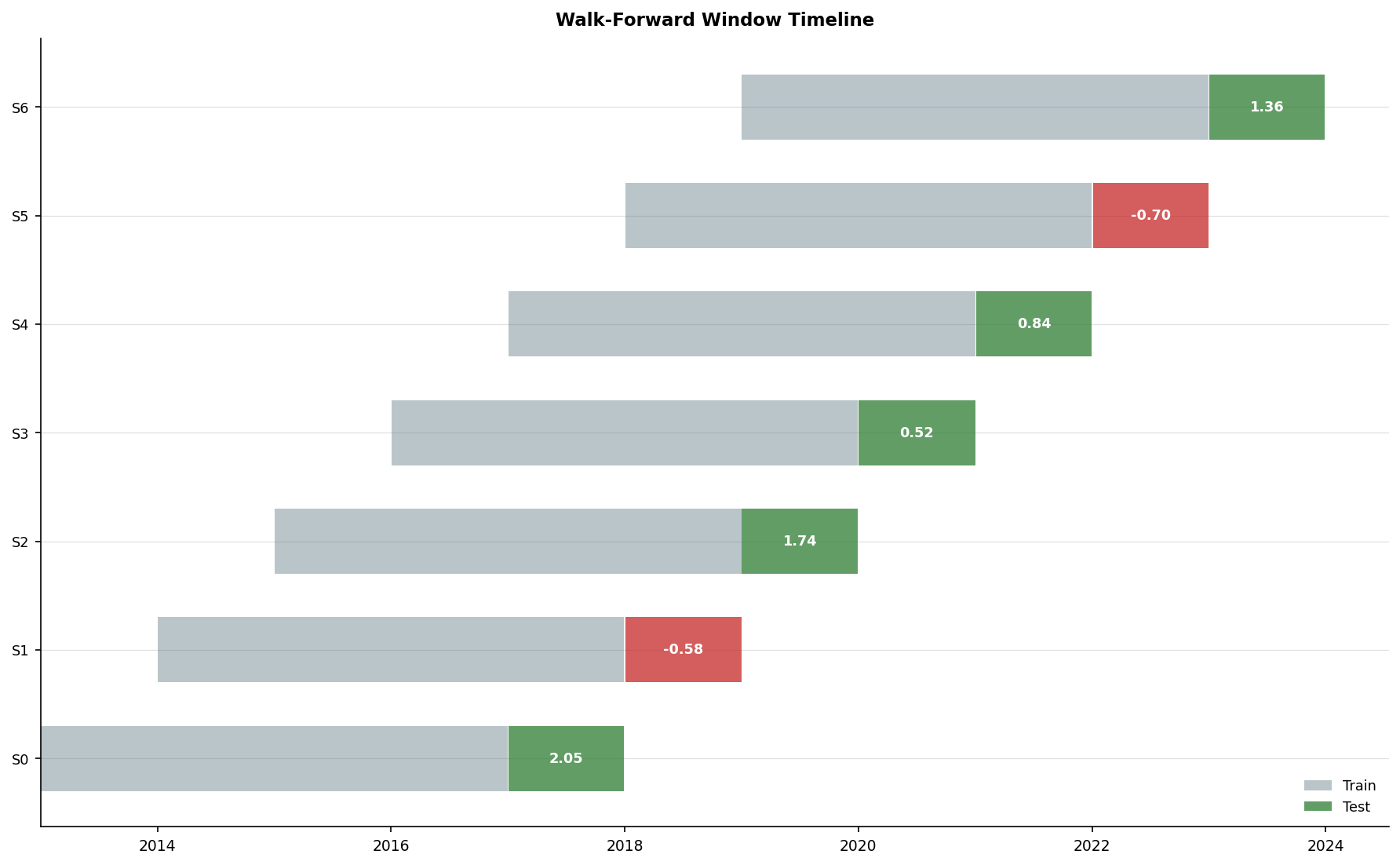
Walk-forward validation divides the research history into a sequence of chronological training and testing windows. For each split, the model is trained using historical observations available up to that point and then evaluated exclusively on the subsequent test period. Once the test period is completed, the training window is advanced and the process repeats.

This procedure ensures that every prediction is generated using information that would have been available at the time the forecast was made. Future information is never incorporated into model estimation, feature construction, or portfolio decisions.

Figure walk_forward_timeline illustrates the validation framework used throughout this research. Each segment represents a distinct train-test cycle, demonstrating how the model is repeatedly retrained and evaluated across multiple market environments spanning the research period.

Walk-forward validation timeline showing chronological training and testing windows.
Figure 07.1 - Walk-forward validation framework. The model is repeatedly trained on historical data and evaluated on subsequent unseen periods, ensuring strict chronological separation between training and testing observations.
07.3

Out-of-Sample Performance

The most important question is whether the strategy continues to generate value when evaluated exclusively on unseen data.

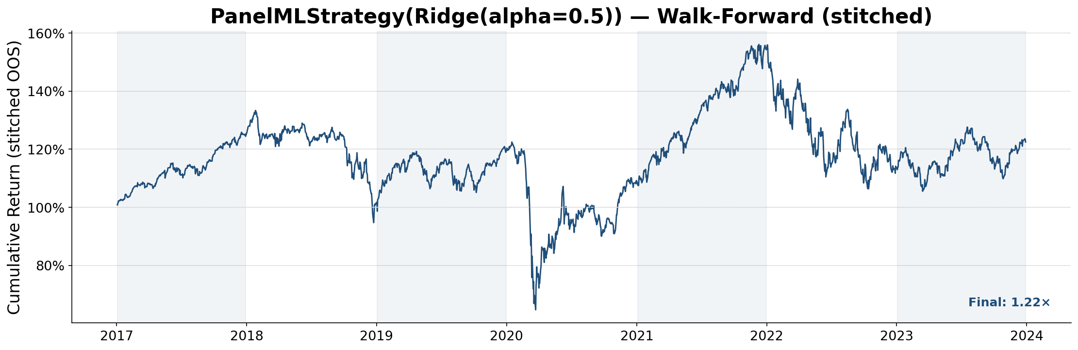
For each walk-forward split, portfolio construction, signal generation, and performance measurement are performed using only information available within the corresponding training period. The resulting out-of-sample returns from all validation windows are then combined into a single continuous performance series.

Figure walk_forward_stitched presents this stitched out-of-sample equity curve. Unlike the historical performance results shown previously, every segment of this curve represents performance generated from predictions made on data that were not available during model training.

This figure therefore provides the most realistic estimate of how the research framework would have behaved under repeated deployment through time. While no historical simulation can perfectly replicate live trading conditions, out-of-sample evaluation provides a substantially more rigorous test of predictive validity than in-sample analysis alone.

Stitched out-of-sample equity curve across walk-forward validation windows.
Figure 07.2 - Stitched out-of-sample equity curve produced by combining the test-period results from all walk-forward validation windows. Every segment represents performance generated on previously unseen data.
07.4

Consistency Across Validation Windows

A positive aggregate out-of-sample result is encouraging, but it does not reveal whether performance was broadly consistent or concentrated within a small number of favourable periods.

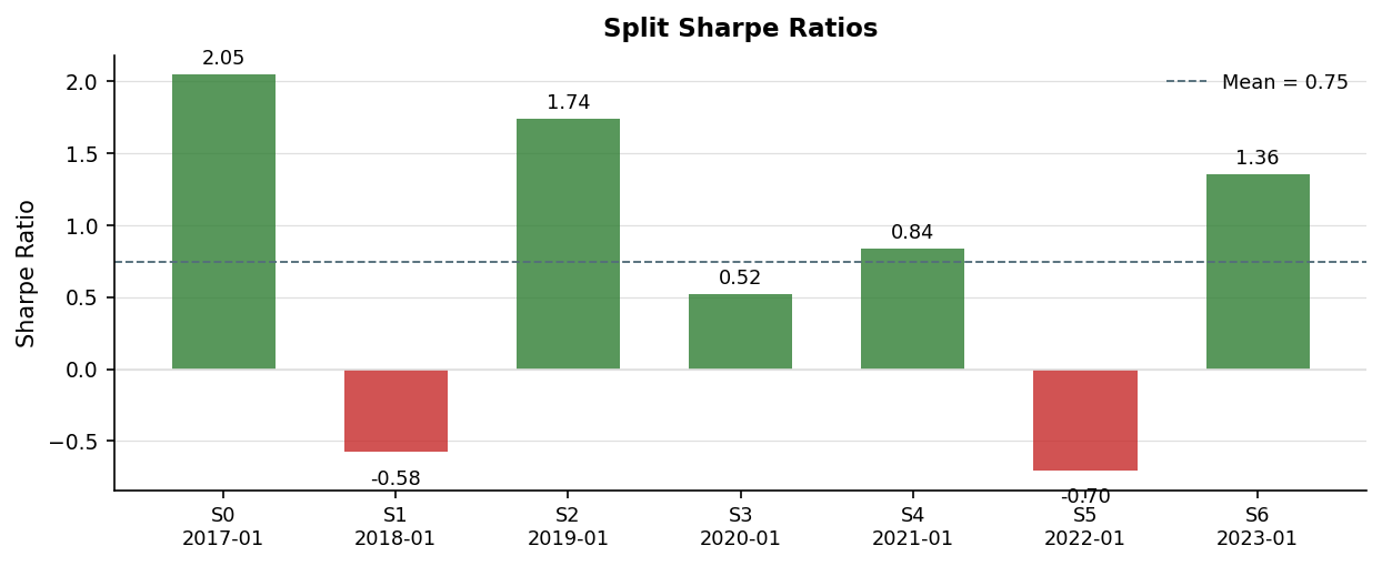
To answer this question, each validation window must be examined individually. If performance is driven by only one or two exceptional periods, confidence in the robustness of the research conclusions should be limited. Conversely, if predictive performance persists across multiple independent test windows, confidence that the signal reflects genuine information rather than random variation is strengthened.

Figure split_sharpes reports the out-of-sample Sharpe ratio achieved within each validation window. Examining results at the split level provides a more granular view of model behaviour and helps identify whether predictive performance remained stable as market conditions evolved through time.

Consistency across independent validation periods is particularly important because the research spans multiple market environments, including periods of expansion, contraction, elevated volatility, and recovery. A signal that survives across diverse conditions is generally more credible than one that succeeds only within a narrow subset of historical circumstances.

Out-of-sample Sharpe ratios for individual walk-forward validation windows.
Figure 07.3 - Out-of-sample Sharpe ratios for individual walk-forward validation windows. Evaluating each split independently helps assess the consistency and robustness of predictive performance across changing market conditions.
Key Takeaway

Historical performance demonstrates what the strategy achieved. Walk-forward validation evaluates whether those results survive exposure to genuinely unseen data.

By repeatedly retraining the model, enforcing strict chronological separation between training and testing observations, and evaluating performance across multiple independent validation windows, the research moves beyond descriptive backtesting toward a more realistic assessment of predictive robustness.

The results indicate that the signal retains economically meaningful predictive power out-of-sample, providing evidence that the relationships identified by the research are not solely artefacts of the historical sample used for model development.

Having established that the signal survives repeated out-of-sample evaluation, the final step is to examine what the validation process revealed about the strengths, weaknesses, and limitations of the underlying predictive framework.

Transition to Section 08

Walk-forward validation provides evidence that the signal retains predictive value beyond the data used for model development. However, validation does more than establish whether a strategy works. It also reveals where performance is strongest, where it weakens, and which aspects of the underlying research framework contribute most consistently to predictive success.

Understanding these behaviours is essential for interpreting the strengths and limitations of the model. The next section therefore moves beyond performance evaluation and examines the research findings that emerged from the validation process, including feature robustness, coefficient stability, and the concentration of predictive power across competing hypotheses.

Diagnostics

08 Research Findings & Limitations

08.1

Beyond Performance Evaluation

The objective of walk-forward validation was not merely to determine whether the strategy generated positive out-of-sample performance. Validation also provides an opportunity to examine how the underlying research framework behaved across changing market environments. By analysing feature behaviour, coefficient stability, and the sources of predictive power, it becomes possible to identify both the strengths of the current approach and the areas where further development may be required.

The focus of this section is therefore not performance itself, but the research findings that emerged from the validation process. Understanding which hypotheses proved robust, which relationships remained stable, and where predictive power ultimately originated provides valuable insight into both the capabilities and limitations of the framework.

08.2

Finding 1: Not All Features Survived Validation

The feature library was deliberately constructed to represent multiple competing hypotheses about market behaviour. Some features were designed to capture trend persistence, others sought to identify mean reversion, volatility dynamics, or structural characteristics of the asset universe. While each hypothesis was theoretically motivated, the ultimate test is whether it contributes predictive information when evaluated on unseen data.

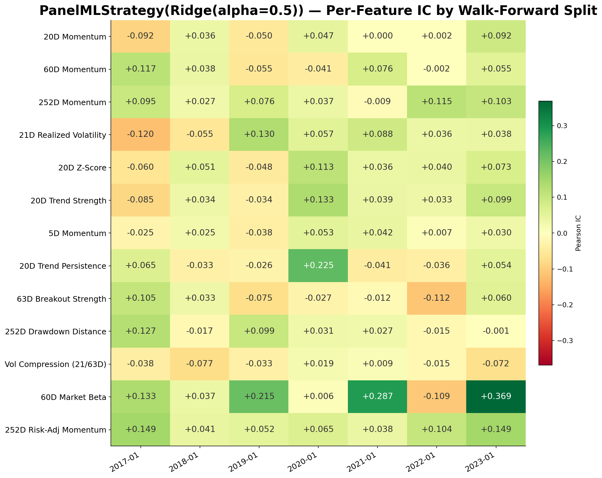
Out-of-sample information coefficient heatmap by feature and walk-forward validation split.
Figure 08.1 - Out-of-sample information coefficients by feature and walk-forward validation split. Positive values indicate that higher feature values were associated with stronger subsequent performance, while negative values indicate the opposite relationship.

Several observations emerge immediately.

First, predictive power is not distributed evenly across the feature library. A relatively small subset of features generates most of the positive information content observed during validation.

In particular, 60D Market Beta, 21D Realised Volatility, and 252D Risk-Adjusted Momentum exhibit the strongest and most persistent positive information coefficients across multiple validation windows. These features continue to contribute predictive information even as market conditions evolve.

Conversely, several hypotheses contribute little or exhibit consistently negative information coefficients. The most notable example is 63D Breakout Strength, which produces negative information coefficients across most validation periods despite being theoretically motivated as a trend-following signal.

This finding is significant because it demonstrates that the validation process acts as a mechanism for feature selection. The research framework successfully identified several robust predictive relationships, but it also revealed that not every engineered hypothesis adds value. Validation therefore helps distinguish durable signals from ideas that appear plausible in theory but fail to generalise out-of-sample.

08.3

Finding 2: Predictive Relationships Were Not Perfectly Stable

A successful prediction system does not necessarily learn the same relationships throughout time. Financial markets evolve continuously, and features that are predictive during one period may become less informative during another. Understanding whether the model relies on stable relationships or continuously changing ones is therefore an important part of evaluating robustness.

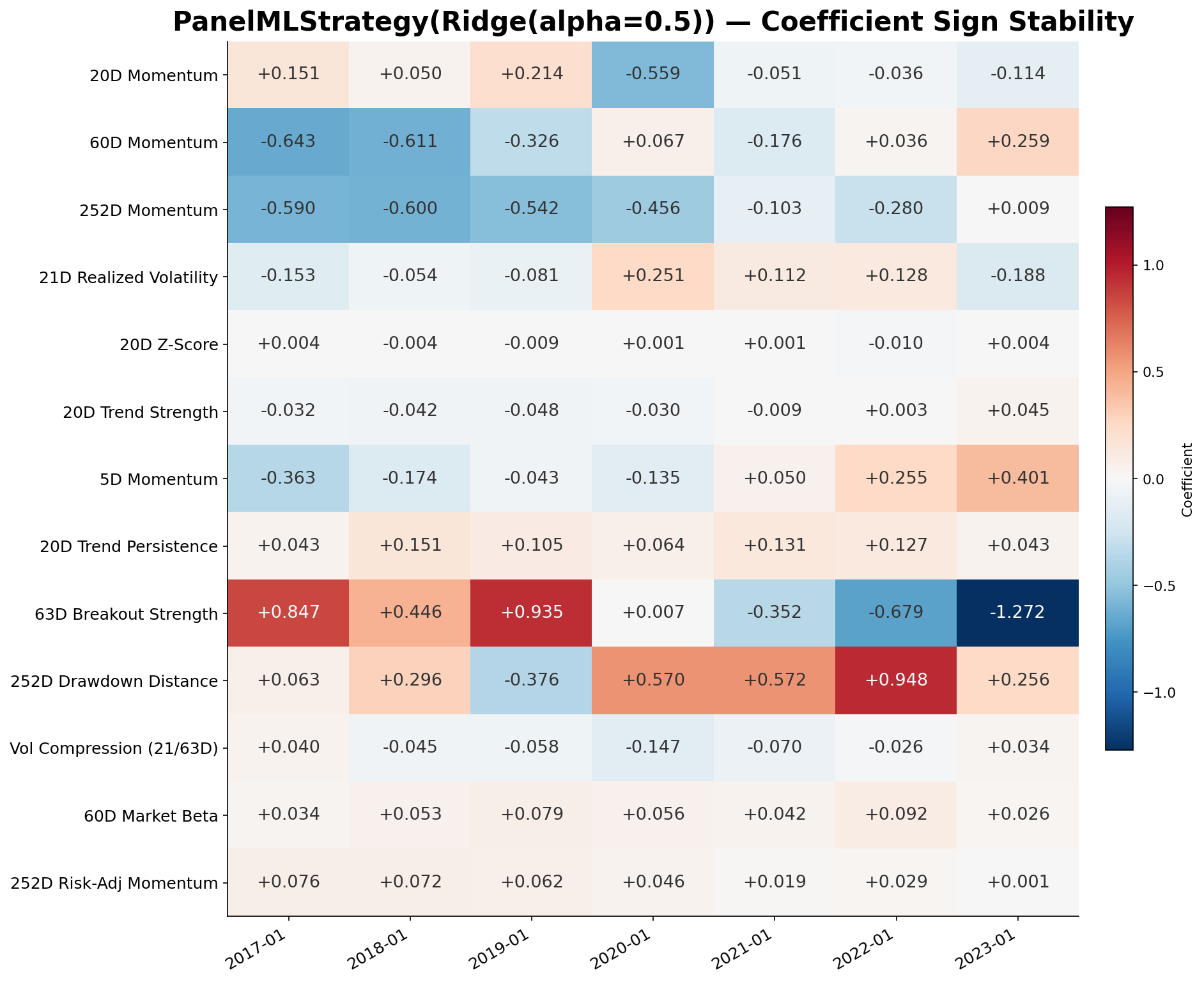
Ridge regression coefficient values by feature and walk-forward validation split.
Figure 08.2 - Coefficient values by feature and walk-forward validation split. Consistent signs indicate stable relationships, while sign changes suggest evolving model behaviour across market environments.

Several relationships remain remarkably consistent throughout the validation period. For example, 60D Momentum remains negative across every walk-forward split, while 60D Market Beta and 63D Risk-Adjusted Momentum maintain broadly stable directional influence.

Other features behave less consistently. Their coefficients fluctuate in magnitude and occasionally reverse sign as market conditions change, indicating that the model adapts its interpretation of certain signals through time.

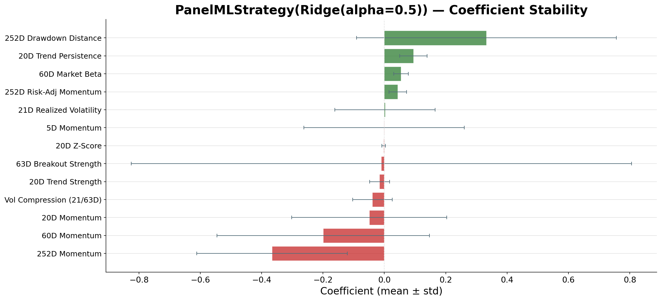
Mean coefficient values with variation across walk-forward validation splits.
Figure 08.3 - Mean coefficient values with variation across walk-forward splits. Larger uncertainty ranges indicate features whose influence changes materially through time.

The stability analysis reinforces this observation. While some features possess meaningful average coefficients, many exhibit substantial uncertainty ranges across validation windows. In several cases the uncertainty exceeds the average effect itself.

This represents one of the principal limitations identified by the research.

The strategy demonstrates economically meaningful predictive power out-of-sample, yet the underlying relationships generating that performance are not perfectly stable. The model is therefore adapting to changing market conditions rather than relying on a single immutable set of relationships.

From a research perspective this is not necessarily undesirable. Financial markets are dynamic systems, and some degree of adaptation is expected. Nevertheless, the results suggest that future improvements should focus on identifying features whose predictive influence remains more stable through time.

08.4

Finding 3: Predictive Power Was Concentrated in Trend Signals

The previous analyses examined individual features. A broader question is whether predictive power was distributed across multiple independent hypotheses or concentrated within a small subset of the research framework.

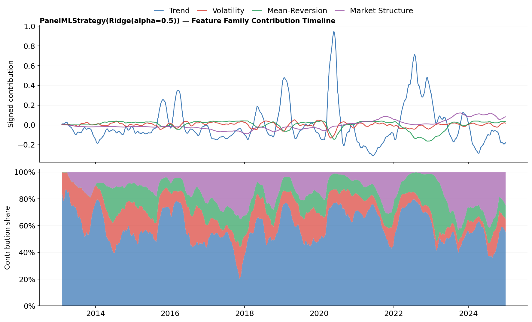
Feature family contribution timeline showing signed contribution and relative share through time.
Figure 08.4 - Contribution of each feature family through time. The upper panel shows signed contribution, while the lower panel illustrates the relative share of total contribution attributed to each hypothesis family.

The contribution profile reveals a highly asymmetric distribution of predictive power.

Trend-related features dominate the research framework throughout most of the sample period. In many periods, trend signals account for the overwhelming majority of total model contribution and frequently represent more than three quarters of the total signal influence.

Mean-reversion signals contribute intermittently, occasionally becoming important during specific market environments, but rarely matching the influence of the trend family. Market-structure signals become increasingly relevant during the latter part of the sample, suggesting that cross-sectional risk characteristics may contain useful predictive information beyond pure price behaviour.

Volatility-related features contribute comparatively little throughout most of the research period.

This finding reveals both a strength and a limitation.

The strength is that the research successfully identified a signal family that consistently contributes predictive information. The limitation is that predictive power is concentrated. The strategy is not drawing equally from multiple independent sources of information. Instead, a large proportion of its performance can be traced back to a relatively narrow subset of trend-related hypotheses.

This concentration creates a clear opportunity for future research. Improving the robustness of mean-reversion, volatility, and market-structure features may increase diversification of predictive information and reduce dependence on a single dominant signal family.

Key Takeaway

Walk-forward validation demonstrated that the strategy retains predictive value out-of-sample. However, the deeper analysis presented in this section reveals that predictive power is neither evenly distributed nor perfectly stable.

A relatively small subset of features generates most of the useful information, the relationships learned by the model evolve through time, and the majority of predictive influence originates from trend-based hypotheses.

These findings are valuable because they provide a clear roadmap for future development. Rather than searching broadly for improvements, subsequent research can focus on strengthening weaker feature families, improving coefficient stability, and diversifying the sources of predictive information that drive portfolio decisions.

Transition to Section 09

The preceding sections have documented the complete research process, from universe construction and feature engineering through prediction, portfolio construction, backtesting, validation, and diagnostic analysis. Together, these stages provide a comprehensive view of both the strengths and limitations of the framework.

The final section synthesises the principal conclusions of the investigation. Rather than examining individual diagnostics or figures, it summarises the most important findings, the key lessons learned throughout the research process, and the most promising directions for future development.

Research Summary & Future Directions

09 Research Summary & Future Directions

09.1

Research Summary

The objective of this research was to investigate whether a systematic cross-sectional machine learning framework could identify economically meaningful differences in future asset performance within a diversified multi-asset ETF universe.

To answer this question, a complete research pipeline was developed encompassing universe construction, feature engineering, prediction modelling, portfolio construction, historical evaluation, walk-forward validation, and diagnostic analysis. Rather than focusing solely on performance outcomes, the research emphasised transparency, reproducibility, and rigorous evaluation throughout the entire research process.

The resulting framework combined a diversified universe of twenty ETFs spanning multiple asset classes with a feature library designed to capture trend, volatility, mean-reversion, and market-structure effects. These signals were transformed into cross-sectional forecasts, translated into portfolio decisions through a disciplined construction framework, and evaluated using strict out-of-sample validation procedures.

The results demonstrate that the framework successfully identified predictive information within the selected asset universe and converted that information into economically meaningful portfolio decisions. More importantly, the signal retained predictive value under repeated walk-forward validation, providing evidence that the observed relationships were not solely artefacts of the historical sample used for model development.

09.2

Principal Findings

Several important conclusions emerged from the research process.

1. Cross-Sectional Asset Ranking Contains Predictive Information

The prediction system consistently generated rankings that exhibited positive information coefficients, meaningful prediction spreads, and broadly monotonic behaviour across ranking groups. Higher-ranked assets generally outperformed lower-ranked assets, indicating that the model successfully captured information relevant to future relative performance.

This finding supports the central hypothesis of the research: cross-sectional machine learning techniques can identify economically meaningful differences in expected asset returns within a diversified ETF universe.

2. Historical Price Information Contains Useful Predictive Structure

One of the most significant findings of the project is that all predictive signals were derived exclusively from historical price information.

No fundamental data, macroeconomic indicators, analyst forecasts, alternative datasets, or proprietary information sources were used. Instead, predictive signals emerged from systematically engineered features designed to capture different aspects of market behaviour.

Despite this intentionally constrained information set, the framework identified relationships that survived both portfolio implementation and out-of-sample validation. The evidence therefore suggests that historical price behaviour contains exploitable structure that can be transformed into predictive signals through disciplined feature engineering and rigorous validation.

While these signals are imperfect and far from sufficient to explain all future market behaviour, they demonstrate that meaningful information exists even within a relatively simple data source when analysed systematically.

3. Validation Confirmed Out-of-Sample Predictive Value

Historical performance alone cannot establish whether a strategy is genuinely predictive. The walk-forward validation framework therefore served as the most important test of research robustness.

The results demonstrated that predictive power persisted across multiple independent validation windows and diverse market environments. While performance varied across individual periods, the framework retained economically meaningful out-of-sample behaviour, increasing confidence that the signal reflects genuine information rather than purely historical noise.

This does not imply that future performance is guaranteed. Rather, it indicates that the relationships identified by the research exhibit a degree of robustness beyond the sample used for model development.

4. Predictive Power Was Unevenly Distributed

The diagnostic analysis revealed that not all engineered hypotheses contributed equally.

A relatively small subset of features generated most of the useful predictive information, while several theoretically motivated features exhibited weak or inconsistent behaviour. Trend-related signals emerged as the dominant source of predictive power, whereas volatility and mean-reversion features contributed less consistently throughout the sample.

This finding highlights the importance of rigorous feature evaluation and demonstrates that successful quantitative research depends not only on generating ideas, but also on systematically validating them and removing those that fail to contribute meaningful information.

5. Stability Remains an Open Challenge

Although the framework demonstrated predictive value, coefficient diagnostics revealed that many learned relationships evolved through time. Certain features remained relatively stable, while others varied materially across validation windows.

This suggests that the model is adapting to changing market conditions rather than relying on a single fixed set of relationships. While such adaptation is expected in financial markets, improving stability remains an important area for future research.

The objective of future development should therefore not simply be to increase performance, but to improve the robustness and consistency of the underlying predictive relationships.
09.3

Research Perspective

This project was intentionally designed as a research programme rather than a search for a single profitable model.

The objective was not to maximise historical performance through repeated optimisation, but to establish a transparent framework capable of generating, evaluating, and refining predictive hypotheses in a disciplined manner. Throughout the investigation, emphasis was placed on reproducibility, out-of-sample validation, diagnostic analysis, and clear separation between research development and performance evaluation.

The resulting framework combines a diversified multi-asset universe, a broad library of economically motivated features, systematic portfolio construction rules, and rigorous validation procedures. Each stage of the process generates evidence that can be inspected, challenged, and refined, allowing research decisions to be evaluated in context rather than in isolation.

Equally important, the framework does not merely reveal what works. It also reveals what does not work. The validation and diagnostic stages identified ineffective features, unstable relationships, and areas where predictive power remains concentrated. These findings are not failures of the research process; they are valuable outcomes that guide future development and reduce the risk of pursuing unproductive directions.

This emphasis on evidence-driven iteration reflects how professional quantitative research evolves in practice. Progress is achieved not through isolated backtests, but through the continuous generation, testing, validation, and refinement of competing hypotheses.

09.4

Future Directions

The findings of this research suggest several opportunities for future development.

Priority areas include:

Expanding the diversity of predictive information beyond trend-dominated signals.

Improving the robustness of mean-reversion and volatility feature families.

Reducing coefficient instability across validation windows.

Exploring alternative portfolio construction and weighting methodologies.

Extending the framework to larger universes and additional asset classes.

Incorporating new information sources alongside price-derived features.

These directions are motivated directly by the evidence generated throughout the research process and provide a clear roadmap for future iterations of the platform.

Final Takeaway

The objective of this project was not simply to build a predictive model, but to establish a disciplined framework for quantitative research.

Throughout the investigation, each stage of the process was designed to transform intuition into evidence. Hypotheses were formalised through feature engineering, evaluated through predictive modelling, tested through portfolio construction, and challenged through rigorous out-of-sample validation. The resulting framework provides a transparent methodology for determining not only whether a signal appears to work, but why it works, where it fails, and how it can be improved.

While the predictive signal identified in this study remains imperfect, the research demonstrates that meaningful information can be extracted from historical market data through a systematic and evidence-driven process. More importantly, it illustrates how quantitative research progresses: not through isolated performance results, but through the continuous generation, testing, validation, and refinement of competing hypotheses.

The value of the framework therefore extends beyond the specific results presented here. It provides a foundation for future investigation and a repeatable process for transforming market observations into testable investment ideas.